Research talk:Reading time/Work log/2018-10-16
Tuesday, October 16, 2018[edit]
Model Selection.[edit]
On Sunday, we observed that although Lognormal and Exponentiated Weibull KS tests passed KS tests. QQ and PP plots revealed that these distributions were not fitting the extreme values very well. These extreme values may not be indicative of reading behavior (e.g. people may leave browser tabs open). However, ideally we will find a model for the whole range of the data instead of choosing an arbitrary cutoff and using a truncated model. I think we have already done a pretty thorough job with model selection here, especially since many of the most interesting questions we would like to answer are about correlations between variables of practical and theoretical interest. However, I was curious as to whether a power-law distribution would fit the data better than the Lognormal and Exponentiated Weibull distributions we have tried so far. So today I added the pareto type-2 distribution (lomax) to the model selection code. Lomax is a 2 parameter power law distribution with support on .
Here is a very good paper by Michael Mitzenmacher explaining data generating processes for power law (pareto) type data generating processes that compares them to log normal distributions. My takeaway is that many types of data generating processes can generate either a log normal or pareto distributions. Rich-get-richer dynamics (preferential attachment) are often associated with power law distributions. However according to Mitzenmacher, multiplicative processes can produce either lognormal or power law distributions, depending on somewhat subtle differences in the process. These both seem somewhat counter-intuitive for reading time. Finally, Mitzenmacher also points out that a mixture of 2 log normal distributions is also a power law. Perhaps we have a situation where we have 2 distributions (reading, leaving the page open) both of which are log normal. If Pareto distributions are a good fit then we might actually prefer a mixture of two lognormal distributions.
| AIC_rank | BIC_rank | ks_rank | ks_pvalue | |||||
|---|---|---|---|---|---|---|---|---|
| mean | median | mean | median | mean | median | mean | median | |
| model | ||||||||
| lomax | 1.880165 | 2.0 | 1.814050 | 2.0 | 2.086777 | 2.0 | 0.252968 | 1.498555e-01 |
| exponweib | 2.148760 | 2.0 | 2.359504 | 2.0 | 1.958678 | 2.0 | 0.279059 | 1.845931e-01 |
| lognorm | 2.173554 | 2.0 | 2.057851 | 2.0 | 2.318182 | 2.0 | 0.255167 | 1.479791e-01 |
| weibull_min | 3.954545 | 4.0 | 3.942149 | 4.0 | 3.917355 | 4.0 | 0.072418 | 3.552921e-05 |
| gamma | 4.958678 | 5.0 | 4.971074 | 5.0 | 4.818182 | 5.0 | 0.041481 | 3.219647e-15 |
| expon | 5.884298 | 6.0 | 5.855372 | 6.0 | 5.900826 | 6.0 | 0.018722 | 0.000000e+00 |
Pretty good! Lomax is the best fit on average according to AIC and BIC, and nearly the best according to the KS statistic (which does not penalize Exponentiated Weibull for having an extra parameter). This suggests that it fits the data about as well as Exponentiated Weibull, but using 1 fewer parameter.
| ks_pass95 | ks_pass97_5 | |
|---|---|---|
| mean | mean | |
| model | ||
| lomax | 0.756198 | 0.818182 |
| exponweib | 0.739669 | 0.789256 |
| lognorm | 0.685950 | 0.756198 |
| weibull_min | 0.227273 | 0.260331 |
| gamma | 0.111570 | 0.123967 |
| expon | 0.049587 | 0.053719 |
The first table looks at the mean and median KS statistics. When we look at the rate at which each distribution passes the KS test at 0.05% and 0.025% confidence levels it actually does the best.
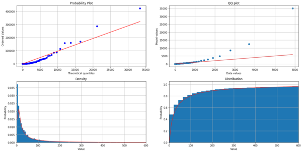
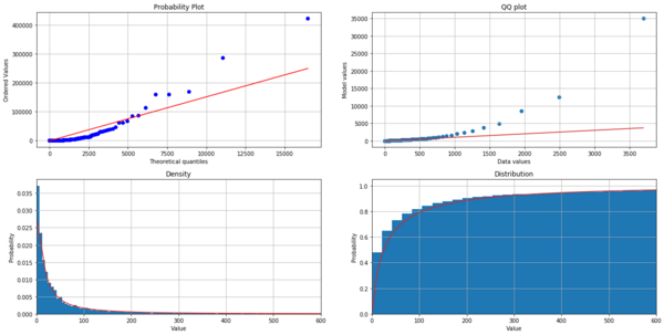
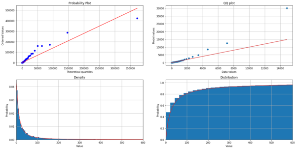
These three plots are useful for comparing the fits of the three parametric models on the data. The lomax does better at fitting the long tail, but it overestimates the probability of short dwell times and underestimates the probably of medium length dwell times.
One important disadvantage to using the Lomax is that the mean is not defined if . Inconveniently, this is the case in about 20% of wikis. We estimated in 77.7% of Wikis.
Maybe Mixture of Lognormals?[edit]
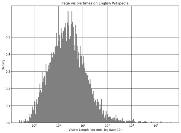
Per Mitzenmacher's point that a mixture of Log Normals may generate a power law, we might explore fitting a mixture model to this data. To take one small step down this path I made a density histogram of the logged visible length.


![{\displaystyle [0,\infty ]}](https://wikimedia.org/api/rest_v1/media/math/render/svg/52088d5605716e18068a460dec118214954a68e9)


